Phase Lock Theory
Created on 2015-04-08 (Wed)
Here I will present the notes I made while developing the phase lock algorithm used to detect trace amounts of DNA orbiting an electrical focal point.It took me some time to wrap my mind intimately enough around the phase lock concept to be able to code it simply into an application. I am going to lay down my thoughts here for my future self to reference.
Phase Locking allows me to hone in on a signal from a noisy source by eliminating all other components of the noisy source except for a known frequency at a known phase. I know the frequency and phase because I either generate the signal or whoever is generating it passes on this information to me. I found that what helped the most was the following mathematical presentation.
Let:
$$ \begin{equation*} \label{eq:equation_1} S_{enc} = A_{enc} \times sin(\omega_{enc} \times t + \theta_{enc}) (1) \end{equation*} $$
be an Encoded Signal. \(S_{enc}\) is composed of the carrier wave and the Signal of Interest I want to transmit across the medium. In this case the amplitude of \(S_{enc}\) varies and is proportional to the Signal of Interest.
Let: $$ \begin{equation*} S_{bkgN} = \sum_{k=1}^n A_k \times sin(\omega_k \times t + \theta_k) (2) \end{equation*} $$
be the Background Noise that accompanies the Encoded Signal. In this case the sum indicates that the profile of the Background Noise spans many frequencies at different amplitudes and phase offsets.
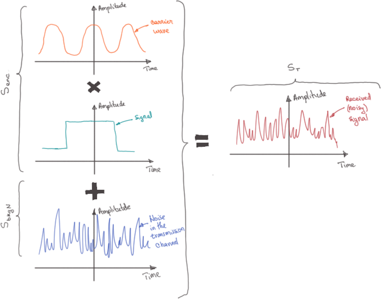
The signal that I receive and that I am going to apply the Phase Lock procedure on contains both the Encoded Signal and the Background Noise: $$ \begin{equation*} \begin{split} S_T &= S_{enc} + S_{bkgN}\\ & =A_{enc} \times sin(\omega_{enc} \times t + \theta_{enc}) + \\ & \phantom{=}\, +\sum_{k=1}^n A_k \times sin(\omega_k \times t + \theta_k) (3) \end{split} \end{equation*} $$
Here is how I imagine the signal of interest, carrier wave and channel noise are combined to result in what gets received by the sensing module:
At this point I am going to delve into a bit of signal processing. My end goal is to extract the amplitude \(A_{enc}\) from the noisy \(S_T\). For this I will use my knowledge that the Encoded Signal \(S_{enc}\) is broadcast at a frequency \(\omega_{enc}\) with a phase offset \(\theta_{enc}\). The procedure is the following:
- Multiply \(S_T\) by a reference signal \(S_{ref}\). In this case \(S_{ref}\) has has the same frequency and phase as \(S_{enc}\).
- Convolve the result by a constant function (this can also be interpreted as integrating the result).
Remember: CONVOLUTION in time domain is MULTIPLICATION in frequency domain. And the other way around.
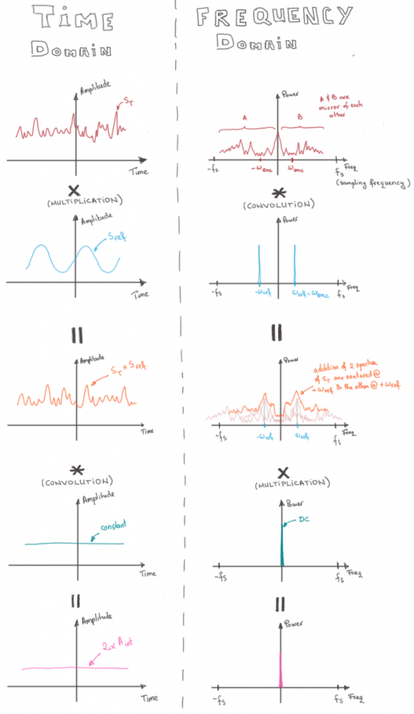
The outcome of the first step (the \(S_T \times S_{ref}\) in the time domain) in the frequency domain is to shift the frequency \(\omega_{enc}\) of my Encoded Signal to DC (0 Hz).
The second step (the convolution of the result of step 1 with a DC function in the time domain) results in all frequencies except DC being multiplied by 0 - practically leaving only the power component of the Encoded Signal.
If you manage to understand the sequence of steps above the math below will make much more sense.
Now that I have a good intuition on what I am planning on doing I'll go through the math in time domain to make sure I get all the fine details right.
So first up is the multiplication - which is also known as "beating" \(S_T\) with a reference signal \(S_{ref}\).
Let: $$ \begin{equation*} S_{ref}=sin(\omega_{ref} \times t + \theta_{ref}) (4) \end{equation*} $$
Then: $$ \begin{equation*} \begin{split} S_T \times S_{ref} &= [A_{enc} \times sin(\omega_{enc} \times t + \theta_{enc})] \times sin(\omega_{ref} \times t + \theta_{ref}) + \\ &\phantom{=}\, +[\sum_{k=1}^n A_k \times sin(\omega_k \times t + \theta_k)] \times sin(\omega_{enc} \times t + \theta_{ref}) (5) \end{split} \end{equation*} $$
Remembering from whatever is left of my trigonometry memories that: $$ \begin{equation*} sin(u) \times sin(v) = \frac{cos(u-v) - cos(u+v)}{2} (6) \end{equation*} $$
The top term of (5) simplifies to: $$ \begin{equation*} \begin{split} \frac{A_{enc}}{2} \times [cos(\omega_{enc} \times t + \theta_{enc} - \omega_{ref} \times t - \theta_{ref}) - \\ - cos(\omega_{enc} \times t + \theta_{enc} + \omega_{enc} \times t + \theta_{ref})] (7) \end{split} \end{equation*} $$
Now remember from the way I chose \(S_{ref}\) that \(\omega_{enc}=\omega_{ref}\) and that \(\theta_{enc}=\theta_{ref}\) so the first \(cos()\) becomes \(cos(0)=1\) which is a DC (non-oscilating) term. So the top term ends up being:
$$ \begin{equation*} \frac{A_{enc}}{2} \times [1 - cos(2 \times ( \omega_{enc} \times t + \times \theta_{enc}))] (8) \end{equation*} $$
The bottom term of (5) becomes: $$ \begin{equation*} \begin{split} \sum_{k=1}^n \frac{A_k}{2} \times [cos(\omega_k \times t + \theta_k - \omega_{ref} \times t - \theta_{ref}) - \\ - cos(\omega_k \times t + \theta_k + \omega_{ref} \times t + \theta_{ref})] (9) \end{split} \end{equation*} $$
In this case however we can't cancel out \(\omega_k \times t\) with \(\omega_{ref} \times t\) unless \(\omega_k\) is equal to \(\omega_{ref}\) and \(\theta_k = \theta_{ref}\). This happens for Background Noise frequencies $\omega_k$ that are “close” to the Encoded Signal \(\omega_{enc}=\omega_{ref}\) frequency and at about the same phase offset \(\theta_k = \theta_{enc} = \theta_{ref}\).
Putting everything together equation (5) can then be simplified to: $$ \begin{equation*} \begin{split} S_T \times S_{ref} &= \frac{A_{enc}}{2} \times [1 -\\ &\phantom{=}\, - \frac{A_{enc}}{2} \times cos(2 \times (\omega_{enc} \times t + \theta_{enc})) + \\ &\phantom{=}\, + \frac{A_k}{2} \times \sum_{k=1}^n cos[(\omega_k - \omega_{ref}) \times t + \theta_k - \theta_{ref}] - \\ &\phantom{=}\, - \sum_{k=1}^n cos[(\omega_k + \omega_{ref}) \times t + \theta_k + \theta_{ref}] (10) \end{split} \end{equation*} $$
Upon a slightly more careful inspection I observe that the result of beating \(S_T\) with \(S_{ref}\) is a DC term and a series of oscillatory terms at different frequencies.
NOTE: Actually there's two DC terms. The 2nd DC term is hidden in the \(cos[(\omega_k - \omega_{ref}) \times t + \theta_k -\theta_{ref}]\) term. This happens as mentioned before when \(\omega_k\) is about the same frequency as \(\omega_{enc}=\omega_{ref}\) and when \(\theta_k\) is equal to \(\theta_{enc} = \theta_{ref}\).
So if I were to filter the result of \(S_T \times S_{ref}\) with a DC filter I would remove all the oscillating terms. To filter using a DC term I convolve the multiplication by a constant term which leaves me with: $$ \begin{equation*} [ S_T \times S_{ref} ] * 1 = \frac{A_{enc}}{2} \times 1 + \frac{A_{k0}}{2} \times 1 (11) \end{equation*} $$
where the \(_{k0}\) term is used to indicate the frequency \(\omega_{k0}\) for which \(\omega_{k0} = \omega_{enc}\) and \(\theta_{k0} = \theta_{enc}\). That is the component of the Background Noise that has a frequency and phase equal (or very close to) the Encoded Signal's frequency and phase.
If we assume the Background Noise at the \(S_{ref}\) frequency and offset is small. Then:
$$ \begin{equation*} [S_T \times S_{ref} ] * 1 = \frac{A_{enc}}{2} (12) \end{equation*} $$
Which means that:
$$ \begin{equation*} A_{enc} = \frac {[S_T \times S_{ref}] *1}{2} (13) \end{equation*} $$
which brings us to the goal of finding \(A_{enc}\).
Thanks to the people at tex.stackexchange (here and here) for teaching me how to use Latex properly.
The biggest thanks go to The Scientist and Engineer's Guide to Digital Signal Processing by Steven W. Smith, Ph.D for teaching me the intro knowledge on convolution.